
要旨
Summary
- PythonライブラリであるJAXを利用することにより、デリバティブ価格計算や金融リスク量計算を容易に高速化できる。
By using JAX, a Python library, you can easily and significantly speed up the calculation of derivative prices and financial risk measures. - CVAやFVAの算出過程で必要なEFV(Expected Future Value)は計算に必要な次元数が多く計算負荷が極めて高い。このEFV計算にJAXを使用して高速に計算する実例を例示(Pythonソース有)。
The Expected Future Value (EFV), which is required in the calculation of CVA and FVA, involves a large number of dimensions and places an extremely high computational load on the system; however, we present a practical example of using JAX to perform these EFV calculations rapidly (Python source code included).
JAXについて
About JAX
JAXは、高性能数値計算および大規模機械学習向けに設計された、アクセラレータ向けの配列計算およびプログラム変換を行うPythonライブラリである。GPU用言語であるCUDAを使わなくても複数GPUをPythonから容易に利用可能になっており、行列演算やモンテカルロ積分等、演算種類によってはCPU利用よりも圧倒的な高速処理を実現できる。
JAX is a Python library designed for high-performance numerical computation and large-scale machine learning, providing array operations and program transformations for accelerators. It allows users to easily utilize multiple GPUs from Python without using CUDA, NVIDIA’s GPU programming language, and can achieve significantly faster processing speeds than CPUs for certain types of computations, such as matrix operations and Monte Carlo integration.
技術的な主な機能を以下列挙。
The main technical features are listed below.
- 演算処理高速化
Acceleration of computational processing- Just In Time compiler- JIT
Pythonで実行時にコンパイルするコンパイラーで、これにより処理速度の高速化を図っている。
It is a compiler that compiles Python code at runtime, thereby improving processing speed. - Accelerated Linear Algebra – XLA
機械学習用にGPU、TPUも利用可能な様にコンパイルする大規模演算向けコンパイラー。CUDAとは異なりハードウェアを意識せず、PythonでGPU、TPUを使用するコードが書ける。
A compiler designed for large-scale computations that compiles code to run on GPUs and TPUs for machine learning. Unlike CUDA, it allows developers to write code in Python that uses GPUs and TPUs without having to worry about hardware specifics. - 自動ベクトル化 Automatic vectorization
ベクトル演算を自動で実装し処理を高速化するプログラミング機能。
A programming feature that automatically implements vector operations to speed up processing. - 自動並列化 Automatic parallelization
複数のGPU、TPUで並列計算を自動で実装し高速化するプログラミング機能。
A programming feature that automatically implements parallel computing across multiple GPUs and TPUs to accelerate processing.
- Just In Time compiler- JIT
- 関数微分
- 自動微分 Automatic differentiation
機械学習におけるバックプロパゲーション用の機能。Pythonで作った関数を自動微分用の関数に渡すとプログラム変換機能で微分係数を取得できる。
CVAやデリバティブ価格を計算する関数を作成すれば、JAXの自動微分実行関数を使用してその関数の微分係数が取得可能。
A feature for backpropagation in machine learning. By passing a Python function to the automatic differentiation function, you can obtain the derivative coefficients using the program transformation feature. If you create a function to calculate CVA or derivative prices, you can use JAX’s automatic differentiation execution function to obtain the derivative coefficients for that function.
- 自動微分 Automatic differentiation
これ等の機能は金融派生商品の価格計算やCVAの計算、センシティビティ(グリークス)
計算等にも有用。
These functions are also useful for calculating the prices of financial derivatives,
calculating CVA, and calculating sensitivities (Greeks).
プレインバニラスワップに対するEexpected Future Value 計算例
Eexpected Future Value Calculation for Plain Vanilla Swaps
(CVA、FVA計算の高速化 Accelerating CVA and FVA Calculations)
CVA、FVAを算出する過程で算出が必要なEexpected Future Value (EFV)は計算量が膨大であり、これがCVA、FVAの計算に時間がかかる大きな要因といえる。1カウンターパーティに対するEFVの計算量は、モンテカルロのパス数、取引件数、タイムグリッド数の3つの積に概ね比例して増加する。ここではプレインバニラスワップのみのカウンターパーティに対するEFV、EPE、ENE計算をJAXとGPUで行い処理時間を確認する。
The expected future value (EFV), which must be calculated during the process of deriving CVA and FVA, involves a massive computational load; this is a major factor contributing to the time required to calculate CVA and FVA. The computational load for calculating EFV for a single counterparty generally increases in proportion to the product of three factors: the number of Monte Carlo passes, the number of transactions, and the number of time grids. Here, we will calculate EFV, EPE, and ENE for a counterparty involving only plain vanilla swaps using JAX and a GPU to verify the processing time.
計算対象 EFV, EPE, ENEの定義
Definitions of EFV, EPE, and ENE for Calculation Purposes
同一カウンターパーティーの、i番目のタイムグリッドtiに対し以下を計算。
For the i-th time grid ti of the same counterparty, calculate the following.
これら計算をタイムグリッド全期間に対し実行。
Perform these calculations over the entire time grid.
計算条件
Calculation Conditions
JAXの効果を示すことが目的のため、計算条件は簡素化する。
To demonstrate the effectiveness of JAX, the computational conditions have been simplified.
- 取引 Trades
- ビジネスデイ、デイカウント等のコンベンションは考慮しない。
Conventions such as business day and day counts are not taken into account. - 取引はプレインバニラスワップのみ。
Plain vanilla swaps only. - 無担保
No margin (collateral). - スワップの変動金利とディスカウントファクターは同じ金利体系
The floating rate on the swap and the discount factor are based on the same interest rate structure.
- ビジネスデイ、デイカウント等のコンベンションは考慮しない。
- 実行条件 Other conditions
- 金利モデル ハル・ホワイト
Interest rate Model: Hull White - 取引件数 1,000件
Number of trades 1,000 - テナー(残存期間) 0.1 – 10年(一様乱数で決定)
Tenor (remaining term): 0.1–10 years (determined by uniform random numbers) - 利払回数 1, 2 or 4回/年 (一様乱数で決定)
Number of interest payments: 1, 2, or 4 times per year (determined by a uniform random number) - タイムグリッド 1/24年
Time Grid: 1/24 Scale - モンテカルロパス数 100,000
Number of Monte Carlo iterations: 100,000 - 使用GPU NVIDIA V100 32GB 1台
1 NVIDIA V100 32GB GPU - データ精度はFP32(C/C++の単精度相当)
Data precision: FP32 (equivalent to single precision in C/C++) - JAX ver0.9.2
- 金利モデル ハル・ホワイト
これ等の条件でCF生成回数はおよそ一千億回となる。
Under these conditions, the number of CF generations will be approximately 100 billion.
実行結果
Execution Results
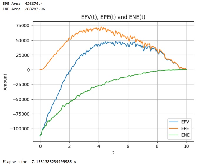
乱数用SEED値により若干の相違が発生するが、古いGPU1台の使用でも上記条件で概ね7秒前後で計算できた。
下図Figure 1 に実行結果のグラフを示す。尚、SEEDを変えれば曲線の形も変わる。
Although there were slight variations due to the random number seed value, even using a single older GPU, the calculation took roughly 7 seconds under the above conditions. Figure 1 below shows a graph of the results. Note that changing the seed value will alter the shape of the curves.
(EPE AREAはEPEの面積、ENE AREAはENEの面積)
ソースコード
Source code
マニュアルベクトル化によるアレイ・プログラミングについて
Array Programming Using Manual Vectorization
今回の例では自動ベクトル化を使用せずアレイ・プログラミングによるマニュアルベクトル化を行っている。 アレイ・プログラミングについてEFVを算出するコードを例示しておく。なお、この例で使用した高速化手法は上述マニュアルベクトル化とJITとXLAの3手法。
In this example, we are performing manual vectorization using array programming rather than automatic vectorization. Below is an example of code that calculates the EFV using array programming. Note that the three optimization techniques used in this example are the manual vectorization described above, JIT, and XLA.
・Python風に記述した一般的なEFV計算コード
General code written in Python style.
for i in range(T):#Time grid
  for j in range(MCpaths):#Monte Carlo Paths
    FVsum = 0
    for k in range(Trades):#Trade
      for l in range(CFs):#Swap CF
        FVsum += CF(i, j, k, l)*DF(i, j, l)
  EFV(i) = FVsum/MCpaths
・JAXを使用したアレイ・プログラミングの疑似コード例(他にも多数の方法が存在)
An example of pseudo-code for array programming using JAX (there are many other methods as well)
for i in range(T):#Time grid
  FVsum =0
  for l in range(CFs):Swap CF
      FVsum += CF(i, l)*DF(i, l) #FVsum.shape=(MCpaths,Trades)
  EFV(i) = sum/MCpaths
実際のコードは”Example of JAX code for calculating EFV”タブに記載。
The actual code is provided in the “Example of JAX code for calculating EFV” tab.
Code for calculating the EFV of a swap using JAX
JAX利用のための環境設定は下記リンク参照。
For information on configuring your environment to use JAX, please refer to the link below.
docs.jax.dev/en/latest/installation.html
尚、GPUがなくてもCPUで計算可能ながら計算時間は数十分かかる。
Note that while the calculation can be performed using the CPU even without a GPU, it will take several tens of minutes.
————————————————————————–
ライセンス表示、初期値
License Notice, Default Values
'''
MIT License
Copyright (c) 2026-present eigenView Inc.
Permission is hereby granted, free of charge, to any person obtaining
a copy of this software and associated documentation files (the
"Software"), to deal in the Software without restriction, including
without limitation the rights to use, copy, modify, merge, publish,
distribute, sublicense, and/or sell copies of the Software, and to
permit persons to whom the Software is furnished to do so, subject to
the following conditions:
The above copyright notice and this permission notice shall be
included in all copies or substantial portions of the Software.
THE SOFTWARE IS PROVIDED "AS IS", WITHOUT WARRANTY OF ANY KIND,
EXPRESS OR IMPLIED, INCLUDING BUT NOT LIMITED TO THE WARRANTIES OF
MERCHANTABILITY, FITNESS FOR A PARTICULAR PURPOSE AND
NONINFRINGEMENT. IN NO EVENT SHALL THE AUTHORS OR COPYRIGHT HOLDERS BE
LIABLE FOR ANY CLAIM, DAMAGES OR OTHER LIABILITY, WHETHER IN AN ACTION
OF CONTRACT, TORT OR OTHERWISE, ARISING FROM, OUT OF OR IN CONNECTION
WITH THE SOFTWARE OR THE USE OR OTHER DEALINGS IN THE SOFTWARE.
'''
import numpy as np
import pandas as pd
import jax
from jax import random
import jax.numpy as jnp
import time
import matplotlib.pyplot as plt
t0 = time.process_time()
#Random Number
seed=12345678
rng0 = jax.random.PRNGKey(seed)
rng0, rng1 = random.split(rng0)
rng1, rng2 = random.split(rng1)
rng2, rng3 = random.split(rng2)
rng3, rng4 = random.split(rng3)
rng4, rng5 = random.split(rng4)
#Trades
n_trades = 1000 #number of transactions
notional = jax.random.randint(rng0, shape=(n_trades,), minval = -100_000, maxval = 100_000)  # Notional
float_rate_current = jax.random.uniform(rng1, shape=(n_trades,), minval = 0.015, maxval = 0.025) #float rate at reference date
fixed_rate = jax.random.uniform(rng2, shape=(n_trades,), minval = 0.01, maxval = 0.03)       # fixed rate
max_remaining_maturity = 10
remaining_maturity = jax.random.uniform(rng3, shape=(n_trades,), minval = 0.1, maxval = max_remaining_maturity) #remaining maturity
freq_type = jnp.array([1, 2, 4])
freq = jax.random.choice(rng4, freq_type, shape=(n_trades,))                # Interest payment frequency
#Parameters
n_paths = 100_000        # Monte Carlo Paths
num_steps_year = 24           # observation times a year
num_steps = num_steps_year * (int(jnp.max(remaining_maturity)) + 1)
dt = (int(jnp.max(remaining_maturity)) + 1.0) / num_steps
## Hull-White
a_HW = 0.1
sigma = 0.0075
r0 = 0.015
# Temporary yield curve for testing purposes
# y(t)=sqrt(coeff_r + r0^2)
coeff_r = 0.0001 #
————————————————————————–
スワッププライシング用関数定義
Function Definitions for Swap Pricing
# Swap revaluation at each point in time
def F0(t): # instantaneous spot rate at time 0. The formula is only for this simulation.
    return jnp.sqrt(coeff_r*t + r0*r0)
def diff_F0(t): #Derivative of instantaneous spot rate curve
    return coeff_r/(2*F0(t))
def f0tT(t, T):  #The forward rate for the period between time t and T as seen at time 0.
    return 2*(F0(T)**3 - F0(t)**3)/((3*coeff_r)*(T-t))

def dicountFactor(t, T, r): #The discount factor for the period between time t and T as seen at time t.
    BtT = (1 - jnp.exp(-a_HW*(T-t)))/a_HW
    AtT = jnp.exp(-f0tT(t, T)*(T-t) + F0(t)*BtT - (sigma**2)/(4*(a_HW**3))*((jnp.exp(-a_HW*T) - jnp.exp(-a_HW*t))**2)*(jnp.exp(2*a_HW*t) - 1))
    BtTr = r[:, jnp.newaxis]*BtT
    df=AtT[jnp.newaxis,:]*jnp.exp(-BtTr)
    return df
def R(t,T, r): #The zero rate for the period between t and T
    return -jnp.log(dicountFactor(t, T, r))/(T-t)[jnp.newaxis, :]
def price_swap(t, r, beginning_pay_date, ):
    def batch_transactions():
        #beginning_pay_date: The first payment date as of the record date
        #first_pay_date: First payment date for each time grid
        n_payment = (jnp.ceil((remaining_maturity - t) * freq)).astype(jnp.int32)
        max_n_payment = jnp.max(n_payment)
        first_pay_date = remaining_maturity - (n_payment - 1)/freq
        float_rate = jnp.where(t < beginning_pay_date, float_rate_current[jnp.newaxis,:], R(first_pay_date-1.0/freq, first_pay_date, r))
        df = dicountFactor(t, first_pay_date, r)
        cf = notional*(jnp.exp(float_rate/freq) - jnp.exp(fixed_rate/freq))
        cfdfsum = cf*df
        def cf_summation(j, price):
            def gen_cf():
                cf_date = first_pay_date + j/freq
                float_rate = R(cf_date - 1/freq, cf_date, r)
                df = dicountFactor(t, cf_date, r)
                cf = jnp.exp(float_rate/freq) - jnp.exp(fixed_rate/freq)
                return notional*cf * df

            cfdf = jnp.where(n_payment > j, gen_cf(), 0)
            price += cfdf #No compensated summation is necessary here.
            return price

        price = jnp.zeros([n_paths, n_trades])
        cfdfsum += jax.lax.fori_loop(1, max_n_payment, cf_summation, price)
        return cfdfsum
    exposure = jnp.where(remaining_maturity > t, batch_transactions(), 0)

    return jnp.sum(exposure,axis=1) #The Compensated summation is necessary here.
————————————————————————–
HWモンテカルロパス生成とタイムグリッド処理
HW MonteCarlo Path Generation and Time Grid Processing
# Interest rate simulation(Euler-Maruyama method)
# dr = (theta(t) - a*r)dt + sigma*dW
def theta(t): #HW Parameter theta
    return diff_F0(t)+a_HW*F0(t)
def find_efv_area():
    r = jnp.zeros((num_steps + 1, n_paths))
    r = r.at[0, :].set(r0)
    norm_rand = jax.random.normal(rng5, shape=(num_steps + 1, n_paths))
    def mc_path(i, ir):
        t = i * dt
        dr = (theta(t) - a_HW*ir[i, :]) * dt + sigma * jnp.sqrt(dt) * norm_rand[i, :]
        ir = ir.at[i+1, :].set(ir[i,:] + dr)
        return ir
    r = jax.lax.fori_loop(0, num_steps, mc_path, r)
    r.block_until_ready()
    n_payment = (jnp.ceil(remaining_maturity * freq)).astype(jnp.int32)
    beginning_pay_date = remaining_maturity - (n_payment - 1)/freq  # The first payment date as of the record date
    efv_epe_ene_list = jnp.zeros([4,num_steps+1])
    def ee_timestep(step, efv_epe_ene_list,):
        step_time = step * dt
        current_r = r[step, :]
        ee = price_swap(step_time, current_r, beginning_pay_date,)
        epe = jnp.maximum(ee,0)
        ene = jnp.minimum(ee,0)
        efv_epe_ene_list = efv_epe_ene_list.at[0, step].set(step_time)
        efv_epe_ene_list = efv_epe_ene_list.at[1, step].set(jnp.mean(ee))
        efv_epe_ene_list = efv_epe_ene_list.at[2, step].set(jnp.mean(epe))
        efv_epe_ene_list = efv_epe_ene_list.at[3, step].set(jnp.mean(ene))
        return efv_epe_ene_list

    efv_epe_ene_list = jax.lax.fori_loop(0, num_steps + 1, ee_timestep, efv_epe_ene_list).block_until_ready()

    df = pd.DataFrame(efv_epe_ene_list.T)
    df.to_csv('EE_EPE_ENE.csv')
    area = jnp.zeros([2])
    def area_summation(i, ar):
        ar = ar.at[0].set(ar[0] + abs(efv_epe_ene_list[2,i] + efv_epe_ene_list[2,i+1])/2*(efv_epe_ene_list[0,i+1]-efv_epe_ene_list[0,i]))
        ar = ar.at[1].set(ar[1] + abs(efv_epe_ene_list[3,i] + efv_epe_ene_list[3,i+1])/2*(efv_epe_ene_list[0,i+1]-efv_epe_ene_list[0,i]))
        return ar
    epe_area = jax.lax.fori_loop(0, num_steps, area_summation, area).block_until_ready()  ##
    print("EPE Area ",epe_area[0])
    print("ENE Area ",epe_area[1])
    return jnp.sum(epe_area), efv_epe_ene_list
————————————————————————–
メイン
Main
if __name__ == '__main__':
    efv_area, ee_epe_ene = find_efv_area()
    efv_area.block_until_ready()
    fig, ax = plt.subplots()
    x = ee_epe_ene[0]
    y0 = ee_epe_ene[1]
    y1 = ee_epe_ene[2]
    y2 = ee_epe_ene[3]
    ax.grid()
    ax.set_title('EFV(t), EPE(t) and ENE(t)')
    ax.set_xlabel('t')
    ax.set_ylabel('Amount')
    ax.plot(x, y0, label='EFV')
    ax.plot(x, y1, label='EPE')
    ax.plot(x, y2, label='ENE')
    ax.legend(loc=4)
    fig.tight_layout()

    plt.show()
    print("Elapse time ",time.process_time()-t0,"s")
上記コードのJupyter Notebook版は以下よりダウンロード可。
A Jupyter Notebook version of the code above is available for download below.
EFV_EPE_ENE_onlySwap_JAX.ipynb
上記例では使用していない自動ベクトル化、自動微分、自動並列化等本件に係る事項にご関心がございましたら以下よりご連絡ください。
Although automatic vectorization, automatic differentiation, and automatic parallelization were not used in the example above, please contact us below if you are interested in specific examples or other details related to this matter.
残課題
Outstanding issues
デリバティブ価格計算、証拠金計算等の全ての計算をPythonコードで記述し直す必要あり。
生成AIを使用して既存のC++コード等からポーティングする方法を検討すると良いかもしれない。
All calculations, including derivative pricing and margin calculations, need to be rewritten in Python code. It might be worth exploring the use of generative AI to port the code from existing C++ code and other sources.